Liquid Water Flow and Retention on the Greenland Ice Sheet in the Regional Climate Model HIRHAM5: Local and Large-Scale Impacts
 Peter L. Langen
 Robert S. Fausto
 Baptiste Vandecrux
 Ruth H. Mottram
 Jason E. Box
- 1Climate and Arctic Research, Danish Meteorological Institute, Copenhagen, Denmark
- 2Geological Survey of Denmark and Greenland, Copenhagen, Denmark
- 3Arctic Technology Centre (ARTEK), Technical University of Denmark, Lyngby, Denmark
To improve Greenland Ice Sheet surface mass balance (SMB) simulation, the subsurface scheme of the HIRHAM5 regional climate model was extended to include snow densification, varying hydraulic conductivity, irreducible water saturation and other effects on snow liquid water percolation and retention. Sensitivity experiments to investigate the effects of the additions and the impact of different parameterization choices are presented. Compared with 68 accumulation area ice cores, the simulated mean annual net accumulation bias is −5% (correlation coefficient of 0.90). Modeled SMB in the ablation area compares favorably with 1041 PROMICE observations with regression slope of 0.95–0.97 (depending on model configuration), correlation coefficient of 0.75–0.86 and mean bias −3%. Weighting ablation area SMB biases at low- and high-elevation with the amount of runoff from these areas, we estimate ice sheet-wide mass loss biases in the ablation area at −5 and −7% using observed (MODIS-derived) and internally calculated albedo, respectively. Comparison with observed melt day counts shows that patterns of spatial (correlation ~0.9) and temporal (correlation coefficient of ~0.9) variability are realistically represented in the simulations. However, the model tends to underestimate the magnitude of inter-annual variability (regression slope ~0.7) and overestimate that of spatial variability (slope ~1.2). In terms of subsurface temperature structure and occurrence of perennial firn aquifers and perched ice layers, the most important model choices are the albedo implementation and irreducible water saturation parameterization. At one percolation area location, for instance, the internally calculated albedo yields too high subsurface temperatures below 5 m, but when using an implementation of irreducible saturation allowing higher values, an ice layer forms in 2011, reducing the deep warm bias in subsequent years. On the other hand, prior to the formation of the ice layer, observed albedos combined with lower irreducible saturation give the smallest bias. Perennial firn aquifers and perched ice layers occur in varying thickness and area for different model parameter choices. While the occurrence of these features has an influence on the local-scale subsurface temperature, snow, ice and water fields, the Greenland-wide runoff and SMB are—in the model's current climate—dominated by the albedo implementation.
Introduction
Greenland ice sheet mass budget changes are among the largest sources of uncertainty in estimates of sea level rise under climate change (Church et al., 2013; Gregory et al., 2013). A key uncertainty in the mass budget is the degree of meltwater retention due to refreezing and capillary forces (e.g., Janssens and Huybrechts, 2000; Harper et al., 2012; Vernon et al., 2013; van As et al., 2016). As the climate has warmed, the zone where melt and rainfall occurs over the snowpack has expanded to higher elevations in the last decade (Howat et al., 2013; de la Peña et al., 2015). Observations from Polashenski et al. (2014) confirm that firn warming is a both long-term (>50 years) and widespread effect. Successive warm summers have also led to the formation of reduced permeability ice lens complexes that expand runoff into the accumulation area, e.g., at the KAN-U site at 1840 m a.s.l (above sea level) in 2012 (Machguth et al., 2016a). Accounting realistically for firn permeability will likely become increasingly important with continued climate warming, and we focus in this paper on representing the pathways of liquid water in snow and firn in a surface mass balance (SMB) model.
When melt or rainfall occurs at the surface of the snowpack, the water typically percolates deeper down and may be stored as liquid water or refrozen in the form of ice lenses (Benson, 1962; Braithwaite et al., 1992). The process by which water percolates in the snowpack was comprehensively described in a Darcian type flow model by Colbeck (1972). Melt percolation has been identified and observed across many glaciers, particularly in the Alps and the Arctic, where deep snow packs often exist overlying glacier ice (e.g., Müller, 1976; Braithwaite et al., 1994; Parry et al., 2007; Wright et al., 2007; Humphrey et al., 2012; Gascon et al., 2013; Polashenski et al., 2014). The meltwater penetration depth is controlled by the temperature and density of the snowpack. Snow/firn density controls the hydraulic conductivity, the pore spaces where water can be contained, and the thermal conductivity of the snow. Subsurface temperature has an important control on densification rate and, via layer cold content, determines if and how much liquid water will freeze.
Once liquid water is in the snowpack, if there is sufficient cold content, the water may refreeze, forming ice layers and pipes. Ice lenses appear to reduce percolation, acting as a barrier to “deep percolation,” i.e., percolation below the previous year's accumulation (Machguth et al., 2016a). Refreezing releases latent heat and acts to warm the snowpack, a phenomenon that has been observed in the Greenland firn over the last 50 years (Polashenski et al., 2014) and seen in modeled snow packs in regional climate simulations (e.g., van den Broeke et al., 2009). However, under high accumulation rate and in locations with low surface slope, meltwater may remain unfrozen and locked in perennial firn aquifers (Forster et al., 2014; Koenig et al., 2014; Kuipers Munneke et al., 2014). Along with refrozen water, perennial firn aquifers have a potentially important delaying effect on sea level rise from Greenland ice in a warming world (Pfeffer et al., 1991). Percolation of meltwater into the snowpack is, however, limited by available pore space (Harper et al., 2012) and future projections by van Angelen et al. (2013) suggest that this pore space may be filled after just a few decades, leading to an acceleration of runoff.
The importance of accounting for these processes has driven the development of snow and firn models within SMB models. As liquid water retention and refreezing are spatially heterogeneous processes and occur at sub-grid scale, early models used parameterizations. Reeh (1989) assumed a fixed percentage of the winter accumulation was retained. Janssens and Huybrechts (2000), Pfeffer et al. (1991) and others developed parameterizations to quantify meltwater retention from a reduced number of variables. Only more recently have meltwater percolation and retention been physically described in firn and snowpack models both at ice sheet scale and in alpine environments (CROCUS, Vionnet et al., 2012; SNOWPACK, Wever et al., 2015). Similar physically-based representations have also been adapted into regional climate models RACMO and MAR (Fettweis, 2007; van den Broeke et al., 2009; Reijmer et al., 2012). The version of HIRHAM5 described in Langen et al. (2015) used a simplified representation of liquid water retention and refreezing.
Declining surface albedo feeding back with temperature and melt plays an important role for the mass balance (e.g., Box et al., 2012; van Angelen et al., 2014). The darkening may be associated both with a general warming (Tedesco et al., 2016) and with increasing amounts of light-absorbing impurities transported to the ice sheet (Dumont et al., 2014; Keegan et al., 2014) or from exposure of “dirty ice” (Tedesco et al., 2016). In any case, the representation of and interplay between albedo processes and subsurface meltwater and refreezing has important effects on the mass balance in a warming climate (van Angelen et al., 2012) including the lower accumulation area (Charalampidis et al., 2015).
In this paper we present results from a HIRHAM5 subsurface scheme which accounts for snow/firn density evolution and hydraulic conductivity and employs two different albedo implementations (described in Section Model Description and Simulations), allowing for formation of firn aquifers and perched impermeable ice layers. In Section Model Evaluation Using Observations, we compare model results to observed net accumulation, SMB in the ablation area, melt extent and subsurface density profiles at multiple ice sheet locations. In addition, we compare simulations with observed subsurface temperature evolution at a single site in West Greenland. We then perform sensitivity tests and discuss the choices made in the model which are particularly important (Section Sensitivity Results). Conclusions are given in Section Conclusions.
Model Description and Simulations
The regional climate model HIRHAM5 combines the dynamical core of the HIRLAM7 numerical weather forecasting model (Eerola, 2006) with physics schemes from the ECHAM5 general circulation model (Roeckner et al., 2003). Details of the configuration are in Christensen et al. (2006). In the all-Greenland domain employed here after Lucas-Picher et al. (2012), HIRHAM5 is run on a horizontal 0.05° × 0.05° rotated-pole grid corresponding roughly to 5.5 km resolution. The atmosphere has 31 levels in the vertical and a 90 s time step. On the lateral boundaries, the ERA-Interim reanalysis (Dee et al., 2011) provides 6 h atmospheric model-level fields of wind, temperature and humidity as well as surface pressure. Across ocean grid points, ERA-Interim sea surface temperatures and sea ice concentration are prescribed. The experiment covers 35 years (1980-2014).
Subsurface Scheme
At the surface, snow mass is updated with snowfall, rainfall, melt and deposition/sublimation at each subsurface scheme time step (1 h). Likewise, the surface temperature is updated via energy budget closure with radiative and turbulent surface energy exchange above and diffusive and advective heat exchange with subsurface layers. If the surface temperature exceeds 0°C, it is reset to 0°C and the excess energy supplies heat for melting (Langen et al., 2015).
The current subsurface model has a number of additions and extensions after the original five-layer ECHAM5 surface scheme (Roeckner et al., 2003) modified for use over glaciers and ice sheets by Langen et al. (2015). Advancements include densification, snow grain growth, snow state-dependent hydraulic conductivity, superimposed ice formation and irreducible water saturation as well as accommodation for water retention in excess of the irreducible saturation. In the following, we describe the details of the new features.
Vertical Discretization
The new subsurface scheme consists of a horizontal grid of non-interacting columns with 32 layers of time-constant water equivalent thicknesses. Each layer's thickness is divided into contributions from snow (ps), ice (pi), and liquid water (pw); each having m w.e. units. While their relative magnitudes can vary through time, the sum of these three parameters equals the layer thickness and remains constant. The layer thicknesses increase exponentially with depth to increase resolution near the surface (N'th layer thickness , with D1 = 0.065 m and λ = 1.173265 chosen to give a full model depth of 60 m w.e. minimizing impacts of lower boundary conditions). The uppermost 2.2 m w.e. are thus represented by 12 layers with thicknesses varying from 6.5 to 37 cm w.e., while the top 10.4 m w.e. has 21 layers with thicknesses up to 1.6 m w.e. The lowest subsurface layer has a thickness of 9.2 m w.e.
As mass is added on top of the subsurface model (via snow, rainfall, condensation or deposition), the scheme advects mass downward to ensure the constant w.e. layer thicknesses. Likewise, when mass is removed from the column by runoff, evaporation or sublimation, mass is shifted up from an infinite ice reservoir below into the lowest model layer. This up- and down mass flux is accompanied by an associated vertical transfer of sensible heat, snow density, grain size and snow, water and ice fractions.
Temperature, Refreezing, and Superimposed Ice Formation
The original ECHAM5 heat diffusion solver (Roeckner et al., 2003) is modified to accommodate a density dependent snow thermal conductivity (Yen, 1981; Vionnet et al., 2012),
where kice is the ice thermal conductivity (in W m−1 K−1) and ρs and ρw are, respectively, the densities of snow and water. The layer bulk thermal conductivity is calculated through a volume-weighted blending of ks and kice. Accumulating snow is assumed to have the temperature of the upper layer, while rain is assumed have 0°C temperature, Tf. The possible energy source from rain with temperature above Tf is thus disregarded. The infinite sublayer, with which the lowest model layer exchanges heat, is set to the simulated local long-term mean near-surface air temperature. This infinite sublayer choice may lead to a slight overestimation of refreezing since the model-bottom will be kept cooler than near-surface layers in case of latent heat release from refreezing. Since the subsurface model is 60 m w.e. deep, the vertical temperature gradient and resulting heat diffusion associated with this bottom cooling will be minor.
The cold content, i.e., the energy required to heat the snow and ice mass to Tf, in each layer is used to freeze liquid water, transferring mass to the ice fraction. Refreezing is assumed to be instantaneous, thereby freezing as much water as is available or as cold content allows within a single time step. The temperature of the layer is raised by latent heat release to conserve energy. Superimposed ice formation occurs when liquid water resides in a temperate layer above an impermeable layer (description below) with a temperature below the freezing point. A downward heat flux at the layer interface is then calculated assuming that the cold, impermeable layer has a linear temperature profile between Tf at the interface and the mean layer temperature at the layer mid-point. This downward heat flux allows superimposed ice to form in the temperate layer and heats the impermeable layer beneath.
Water Saturation
The water saturation, Sw, is the volume of water per pore space volume and may be written in terms of masses as
where ρi = 917 kg m−3 is taken to be the density of ice and pw and ps are the layer masses of water and snow. The maximum water saturation that can be sustained by snow grain capillary tension is termed the irreducible water saturation, Swi, with values employed in models varying widely. Colbeck (1974) found a value of 0.07 experimentally and Yamaguchi et al. (2010) found a value of 0.02, both for snow with a density of about 550 kg m−3. Coleou and Lesaffre (1998) experimented with variable densities and found an approximate relationship between porosity, P = 1−ρs/ρi, and the water per snow-plus-water mass irreducible liquid water content, Wmi:
The quantity Wmi may be converted to Swi through the relation
As ρs increases, Swi calculated in this manner initially decreases from ~0.10 at 100 kg m−3 to ~0.07 at 300 kg m−3. Swi then increases to about ~0.085 at 600 kg m−3 and ~0.17 near 810 kg m−3 (Figure 1).
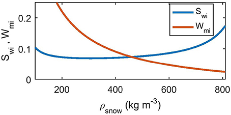
Figure 1. Irreducible saturation, Swi, and irreducible liquid water content, Wmi (water per snow-plus-water mass), as a function of snow density following the parameterization by Coleou and Lesaffre (1998).
Vionnet et al. (2012) used an irreducible water saturation value of 0.05 in the Crocus/SURFEX model. As described by Reijmer et al. (2012), SOMARS/RACMO used 0.02 while Crocus/MAR used 0.06. Kuipers Munneke et al. (2014) used the Coleou and Lesaffre (1998) approach in their study of perennial firn aquifers with the Ligtenberg et al. (2011) firn model. To test the sensitivity toward this choice, we perform experiments with a fixed value of 0.02 along with values calculated based on the Coleou and Lesaffre (1998) parameterization.
Finally, given values of Sw and Swi, we may calculate the effective liquid saturation,
which becomes positive when the snow contains more water than can be permanently held by capillary forces alone.
Downward Flow of Liquid Water
In our treatment of vertical flow of liquid water through the snowpack, we closely follow the implementation by Hirashima et al. (2010). The governing equation for water flow, q (m s−1), is Darcy's law,
where dh/dz is the vertical gradient in capillary suction, h (m units), and the second term (+1) represents gravity. The vertical coordinate, z, increases downwards. The hydraulic conductivity, K (m s−1), and the capillary suction are parameterized in terms of snow grain diameter, dg (mm units), effective liquid saturation, Θ, and snow density, ρs, as follows. The hydraulic conductivity of snow is the product of the saturated and unsaturated conductivities, Ksnow = KsKr, the former of which was determined by Shimizu (1970) to follow:
Here, g is the acceleration due to gravity and νw is the kinematic viscosity of water (1.787·10−6 m2 s−1). Note that dg has mm units. We thus divide by 1000 to get the diameter in m units in accordance with Calonne et al. (2012). In the van Genuchten (1980) parameterization of Kr and h used by Hirashima et al. (2010), two parameters (α and n) must be calculated,
With these, and the quantity m = 1−1/n, we calculate,
As the layers in our subsurface model contain both snow and ice, we need to take into account the hydraulic conductivity reduction resulting from the presence of ice. Colbeck (1975) developed an analytical model for a snowpack with interspersed ice layers, and we employ it here for model layers with some ice fraction. The bulk hydraulic conductivity of the entire model layer is
where fsnow = Hs/(Hs+Hi) is the fraction of the physical layer thickness which is snow (here, Hs = psρw/ρs and Hi = piρw/ρi are the physical thicknesses of the snow and ice fractions). The hydraulic conductivity of ice, Kice, is assumed zero, and the fraction wh/wice is the ratio between the width of holes in the ice and the width of the ice. A value of 1 for this fraction means that when ice is present in a layer, it has a horizontal extent of half the unit area. Here, it is essentially a tuning parameter that can decrease the hydraulic conductivity in the presence of ice and we perform experiments with wh/wice values of 1 and 0.1.
Hirashima et al. (2010) introduced an implementation of Darcy's law that allows for longer time-steps at the cost of considering only downward flow, and the same is adopted here. The instantaneous flux, q0, evaluated using beginning-of-time-step values for all the above quantities influencing K and h, will change during a long time step and taking q0Δt as the time-step total flux will be an overestimate; the total flux into a given layer will at most equal all the water beyond irreducible saturation in the layer above, or it will equal the amount that increases the vertical h-gradient sufficiently to obtain balance between the two terms in Darcy's law (Equation 6). That limiting amount, qlim, is estimated iteratively and allows for calculation of the time-step integrated flux (Hirashima et al., 2010).
During our sensitivity experiments, we also employ a “NoDarcy” version of the code which ignores the delaying effect of hydraulic conductivity on the vertical flow, allowing all water in excess of the irreducible saturation to fully percolate within a single time step.
Impermeable Layers and Runoff
A layer is considered impermeable if its bulk dry density,
exceeds a threshold of 810 kg m−3. This value is lower than the classical value of pore close-off density at 830 kg m−3 (Cuffey and Paterson, 2010), since field studies (Gregory et al., 2014) show that in high-accumulation areas such as West Antarctic Ice Sheet (WAIS) divide (and presumably Greenland), impermeability occurs over a range of densities (780–840 kg m−3) centered around an average of 810 kg m−3. No water is allowed to flow to an impermeable layer from above and the same applies if a layer has its entire pore space filled (Sw = 1). For a layer above an impermeable layer, water that would otherwise have flowed downwards, through either the Darcy or NoDarcy mechanisms described above, becomes available to run off. However, it does not run off immediately. Instead, runoff, QRO, per time-step is calculated from the water in excess of the irreducible saturation, pliqex, as:
where τRO = cRO, 1 + cRO, 2exp(−cRO, 3S) is a characteristic local runoff time-scale that increases as the surface slope, S (unit m m−1), tends to zero (Zuo and Oerlemans, 1996). The coefficients cRO, 1, cRO, 2 and cRO, 3 are set to 0.33 day, 25 days and 140, respectively (as in CROCUS/MAR, Lefebre et al., 2003). With this delayed runoff, water in excess of irreducible saturation may linger in a layer until it forms superimposed ice on the layer beneath, runs off or refreezes.
There is currently no representation of horizontal flow or routing of meltwater in HIRHAM5. Once water runs off as described above, it exits the model domain.
Densification and Grain Growth
Re-writing Equation (5) in Vionnet et al. (2012), the time evolution of the snow density, ρs, is given as
where σ is the overburden pressure and η is the snow viscosity, parameterized as in Vionnet et al. (2012) Equation (7):
Here, kg s−1, aη = 0.1 K−1, bη = 0.023 m3 kg−1, cη = 250 kg m−3 are identical to Vionnet et al. (2012), while f2 is taken to be a constant of 4, neglecting the reduction in η for grain sizes smaller than about 0.3 mm. The effect of liquid water on viscosity and compaction rate enters in f1 as,
Freshly-fallen snow has an initial density parameterized through a linear regression of surface density observations onto surface elevation, zsrf (m a.s.l.), latitude, φ (degrees north), and longitude, λ (degrees east):
with aρ = 328.35 kg m−3, bρ = −0.049376 kg m−4, cρ = 1.0427 kg m−3 deg−1 and dρ = −0.11186 kg m−3 deg−1 (Fausto et al., in preparation).
The snow grain size diameter, dg (in mm), used in the calculation of hydraulic conductivity is modeled following Katsushima et al. (2009) and Hirashima et al. (2010) in terms of the mass liquid water content in percent, L = pw/ps×100, as
The first option, increasing with L3, follows Brun (1989) for low liquid water content, while the second option depends only on the factor. As in Katsushima et al. (2009), we choose an initial value of 0.1 mm for the grain size diameter of freshly fallen snow.
Experimental Design
We perform sensitivity tests with multiple subsurface scheme versions and parameter settings, running the subsurface scheme offline from the HIRHAM5 atmospheric code by saving 6 h fields of surface fluxes of energy (downward short- and longwave radiation, latent and sensible heat fluxes) and snowfall, rainfall and sublimation mass fluxes from HIRHAM5. These fields are in turn read in to the offline subsurface code and interpolated to the 1 h time step employed there. The upward short- and longwave fluxes are calculated in the offline code based on albedo (see below) and surface temperature. Spin-up of the subsurface model is performed by taking an initial condition from a previous experiment and repeating the decade 1980-1989 (chosen since it precedes the warming in later decades) until transients in decadal means of runoff and subsurface temperatures have ceased, typically 50–100 years. A separate spin-up is performed for each sensitivity experiment. After spin-up, the transient 1980-2014 experiment is started from the final model state.
Surface albedo is crucial to determining melt energy and in turn the supply of subsurface liquid water and runoff. We perform sensitivity tests with two different implementations: (i) MODIS-derived daily gridded fields of observed surface albedo after Box et al. (2012, see Section Observational Data), hereafter “MOD,” and (ii) surface albedo computed internally as in Langen et al. (2015), hereafter “LIN” referring to the linear function of temperature. The internally computed albedo thus employs a linear ramping of snow albedo between 0.85 below −5°C and 0.65 at 0°C for the upper-level temperature. The albedo of bare ice is constant at 0.4. Ice and snow albedos are blended for small snow depths using an exponential transition with an e-folding depth of 3.2 cm (as in Oerlemans and Knap, 1998).
Table 1 lists the sensitivity experiments with different combinations of albedo, water percolation mechanism, parameterization of Swi and choice of wh/wice. The experiments MOD-ref and LIN-ref, corresponding to a model with Darcy flow, Swi parameterized following Coleou and Lesaffre (1998) and wh/wice set to 1 (with either MODIS-derived or internally calculated albedo), are considered the reference setting.
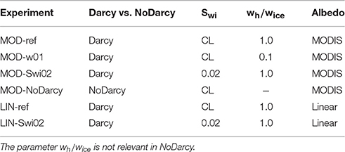
Table 1. Overview of sensitivity experiments with different choices of albedo implementation (MODIS-derived or linear formulation), water percolation mechanism (Darcy or NoDarcy), parameterization of irreducible water saturation, Swi (fixed value of 0.02 or Coleou and Lesaffre, 1998, parameterization) and choice of wh/wice (used in Equation 11).
Model Evaluation Using Observations
In the following, we compare simulated and observed surface accumulation, SMB and surface melt day counts (Section Surface Mass Balance and Melt Extent) as well as subsurface temperature development at a single Programme for Monitoring of the Greenland Ice Sheet (PROMICE) site and subsurface density profiles at a collection of sites (Section Subsurface Temperature and Density). Throughout this study, we use the term SMB for the sum of surface accumulation and ablation, including internal accumulation within the surface snowpack due to refreezing and superimposed ice formation. We note that this term is sometimes also referred to as climatic mass balance (e.g., Cogley et al., 2011). The surface accumulation (and to some extent also ablation) is external to the subsurface model in the sense that accumulation is provided exclusively from the HIRHAM5 atmospheric model. The ablation is a result of the downward energy fluxes from HIRHAM5, but also the albedo calculated in the LIN simulations and specified in the MOD simulations at the top of the subsurface model. It furthermore depends on the subsurface energy flows and thus also on the other model choices.
Observational Data
MODIS Albedo
The Moderate Resolution Imaging Spectroradiometer (MODIS) MOD10A1 surface albedo used in the model is de-noised and smoothed as described by Box et al. (2012), whereby residual cloud artifacts are identified and rejected using running 11-day statistics in each pixel. Values that differ by more than two standard deviations from the 11-day mean are rejected unless they are within 0.04 of the median. Finally, the 11-day running median is used as the daily value. Given that data are only available since 2000, a daily MODIS-climatology based on the pre-darkening period 2000-2006 (see Tedesco et al., 2016) is used prior to 2000 (as in Fausto et al., 2016b).
Accumulation
A compilation of 86 ice cores providing annual w.e. net accumulation rate is available from Box et al. (2013), and spans elevations between 311 and 3188 m a.s.l. Here we select cores overlapping in time with our experiments and having elevations above 1000 m a.s.l. This gives a total of 68 cores (red circles in Figure 2 and Supplementary Table S1) providing a sample across elevations and east-west and north-south differences.
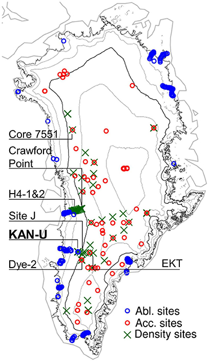
Figure 2. The position of the 68 ice cores used for accumulation evaluation (red circles), 351 SMB observation sites in the ablation area (blue circles) and 75 firn cores used in density evaluation (names of 7 sites included in Figure 7 are shown) with elevation contours (1000-3000 m a.s.l. in steps of 500 m with 2000 m a.s.l. highlighted) and outline of the contiguous ice sheet.
Surface Mass Balance
Historical and contemporary SMB observations from all regions of Greenland compiled by Machguth et al. (2016b) under PROMICE are compared to daily simulated SMB. We use observations that overlap with our experiments and exclude sites that fall outside the model's glacier mask. The selection yields 1041 observations from 351 sites (blue circles in Figure 2). The time span of the SMB observations varies from months to years, although a full year or a 3-month ablation season are the most common. In our analyses (see Table 2 and Figure 4) these observations (in m w.e.) of varying time span enter with equal weights.
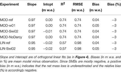
Table 2. Statistics of comparison between 1041 observed (Machguth et al., 2016b) and simulated SMBs from 351 ablation area sites.
Automatic Weather Stations
Interpretation of model-observation discrepancies is aided by the use of automatic weather station data from the PROMICE network (Ahlstrøm et al., 2008, see Supplementary Table S2). From these stations we use near-surface air temperature, surface temperature, downwelling longwave, downwelling shortwave, net incoming shortwave and albedo.
Surface Melt
We use the MEaSUREs Greenland Surface Melt Daily 25 km EASE-Grid 2.0 data set (Mote, 2014) from 1988 to 2012 to compare with modeled melt extent. After 1987, the product has daily resolution and derives from brightness temperatures measured with the Special Sensor Microwave Imager (SSM/I) and Special Sensor Microwave Imager/Sounder (SSMIS) on board Defense Meteorological Satellite Program (DMSP) satellites. Measured brightness temperatures are compared to thresholds found using a microwave emission model to simulate brightness temperatures of a melting snowpack (Mote and Anderson, 1995; Mote, 2007). The result is a daily melt or no-melt field on the 25 km resolution Equal-Area Scalable Earth (EASE) grid.
Subsurface Temperature
Subsurface temperatures were recorded at the western ice sheet percolation area PROMICE site KAN-U (67.0003 N, 47.0243 W, marked in bold in Figure 2) 1840 m above sea level. The station has a thermistor string measuring subsurface temperature to 8–10 m depth (Charalampidis et al., 2015) and we use temperatures interpolated linearly between the thermistors. The depth of each sensor is calculated from maintenance reports and observed surface height changes from acoustic height sensors on the station boom and on a stake assembly few meters away. Between May and August 2012, the stake assembly tilted severely and the station was standing on (and lowering along with) the surface meaning that neither of them could monitor ablation accurately. For that period, we use five firn cores drilled at KAN-U in May 2012 and April 2013 and derive surface lowering between those two dates as the vertical offset that maximizes the correlation of their density profiles (Machguth et al., 2016a).
Density
Simulated subsurface density is evaluated against field measurements using a total of 75 firn cores spanning 1989 to 2013 (green crosses in Figure 2 and Supplementary Table S4). This dataset comprises 14 cores from the Arctic Circle Traverse 2009 to 2013 (Machguth et al., 2016a), 32 cores from the PARCA campaigns in 1997-1998 (Mosley-Thompson et al., 2001), one core drilled at Site J in 1989 (Kameda et al., 1995) and 28 cores from 2007 to 2008 along the EGIG line (Harper et al., 2012). Resolution and accuracy vary for each dataset and are detailed in the studies above. Each core was compared to the modeled density profile of the grid cell it is located in. Different cores can therefore be compared to the same modeled density profile and illustrate within-cell variability of firn density.
Surface Mass Balance and Melt Extent
The observed annual w.e. net accumulation rates compare with simulated net accumulation (calculated in the model as snowfall-minus-sublimation) with an average model bias of −5%, correlation coefficient of 0.90 and orthogonal linear regression slope of 1.01 indicating that the average magnitude and spatial variations are reliably reproduced by the model (Figure 3). Biases are locally both positive and negative and nearly cancel out in the mean but give a 25% root-mean-square-error, with no clear pattern in the distribution of positive and negative biases with elevation.
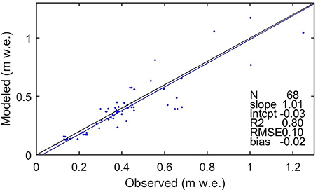
Figure 3. Comparison of modeled and observed annual net accumulation (snowfall-minus-sublimation) for 68 ice cores with elevation greater than 1000 m a.s.l. The black line is 1:1 and the blue line is an orthogonal linear regression with statistics of the fit provided in the table. These are unitless except RMSE and bias (m w.e.).
Figure 4 and Table 2 compare the Machguth et al. (2016b) SMB measurements to nearest-neighbor interpolated simulated daily SMB sums over the dates reported in the observations. The MOD-ref experiment compares favorably with observations (slope 0.97, intercept 0.00 m w.e., R2 0.74 and relative bias −3%, i.e., underestimated net mass loss). The LIN-ref experiment compares almost as well (slope 0.95, intercept −0.02 m w.e., R2 0.57 and relative bias −3%). Comparing across model versions using MOD albedo in Table 2, they are all similar and no clear winner may be identified. The same applies across the two LIN albedo experiments.
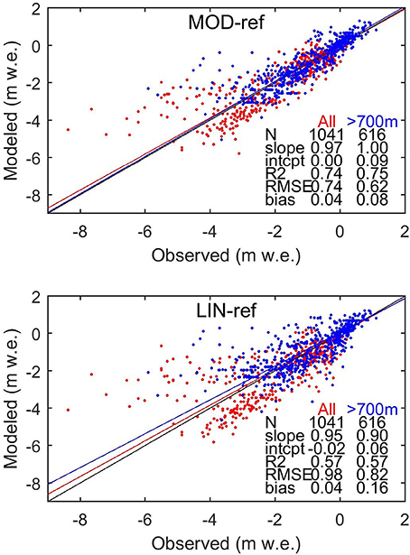
Figure 4. Comparison of modeled and observed SMB at 351 ablation area sites providing a total of 1041 observations. Red dots are at sites below 700 m a.s.l. and blue above 700 m a.s.l. The red line (and the statistics in the “All” column) is an orthogonal linear fit to all 1041 observations, while the blue line is for sites above 700 m a.s.l. The statistics of the fits provided in the tables are unitless except RMSE and bias (m w.e.). The black line is 1:1. Units on the axes are in m w.e. and the observations cover uneven time intervals: some are a few months, some are 1 year and some are 2 years. Model numbers are integrated over the exact dates of the observation intervals.
To investigate the elevation dependence of the SMB comparison, statistics are redone for sites above and below 700 m a.s.l. (above 700 m shown in blue in Figure 4). At high elevation sites, the MOD-ref and LIN-ref experiments on average underestimate the net mass loss by 8 and 16%, respectively. At low elevation sites, they overestimate net mass loss by 1 and 7%, respectively. The small negative bias found for all sites (−3%), is thus a result of cancelation of under- and overestimates at high and low elevation sites. To gauge the overall impact of the low- and high-elevation biases, we calculate the total long-term runoff deriving from elevations above and below 700 m a.s.l. in the MOD-ref and LIN-ref experiments. We find that in both experiments, about 38% of the total ice sheet-wide runoff derives from below 700 m a.s.l. Considering the biases (+1 and +7% at low elevations for MOD and LIN, and −8 and −16% at high) together with 38% runoff from low areas and 62% from high, suggests weighted mean ice sheet-wide mass loss biases in the ablation area of −5 and −7% for the MOD and LIN cases, respectively.
For the very largest negative observed SMBs, the model has a pronounced tendency to underestimate the mass loss, see e.g., the leftmost points in both panels of Figure 4 corresponding to the PROMICE QAS_L site in southern Greenland [see Supplementary Table S2). In fact, considering solely the lower ablation area PROMICE sites (KAN_L, KPC_L, NUK_L, NUK_N, QAS_L, SCO_L, TAS_L, and UPE_L, situated at 468 ± 240 m a.s.l. (mean ± stddev)] yields mean underestimates of 29 and 37% for MOD and LIN, respectively.
Reasons for the significant ablation underestimation at very low-elevation sites include: (i) The 5.5 km grid size which cannot resolve some fine-scale land-ice differences near the lowest sites (e.g., QAS_L); (ii) Jun-Aug observed vs. HIRHAM5 near-surface air temperatures at the L-sites indicate simulated cold biases of 2–3 degrees (Supplementary Table S3) giving biases in the air-to-surface temperature contrast typically of similar magnitude (ΔT bias Supplementary Table S3), which are expected to yield underestimated sensible heat input to the surface; (iii) A simplistic representation of surface roughness elements (crevasses, sub-grid undulations) may lead to underestimation of boundary layer turbulence and turbulent heat transfer (Fausto et al., 2016a,b); (iv) Average simulated albedo is overestimated at the low-level sites (Langen et al., 2015; Fausto et al., 2016b) as also shown in Supplementary Table S3. In the LIN case, the fixed bare-ice albedo of 0.4 is too high for sites like QAS_L where, for instance, July 2012 had an average in situ albedo of 0.21 (van As et al., 2013). Even in the MOD case, such a low value is not captured on the HIRHAM5 grid with a mean July 2012 value of 0.44 (Fausto et al., 2016b). Comparing Jun-Aug mean observed and simulated net incoming shortwave radiation (incoming minus reflected) over 2008-2014, QAS_L has model biases of −16 and −44% for MOD and LIN, respectively, as a result of positive mean albedo biases of 0.16 and 0.34 (Supplementary Table S3).
The U-sites also display a tendency for simulated near-surface air temperature cold biases but these are generally smaller than at the L-sites. At the KPC_U site (Northwest Greenland), however, where particularly the LIN case overestimates mass loss, there is a Jun-Aug mean 1.7 degree warm bias. The warm conditions allow a positive feedback between warming surface snow and lowered albedo to be activated resulting in a positive net incoming shortwave bias of 41%. Such a feedback is not active with the specified MOD albedo resulting in a small (−5%) net shortwave bias.
The 1988-2012 brightness temperature-derived melt days are compared to the simulations on the 25 km EASE grid to avoid artifacts of comparison of smoothly varying observations to finer scale variations in the model. Daily simulated fields of melt (value 1) vs. no-melt (value 0) on the 5 km HIRHAM5 grid (defined by daily total melt above 5 mm w.e. as in MAR and RACMO) are bi-linearly interpolated to the 25 km EASE grid and the resulting fractional (0–1) field is converted to melt vs. no-melt using a threshold of 0.5. Counting the melt days annually gives 25 2D fields which are compared between observations and simulations in cells where both have ice. In Table 3, “Bias” shows the long-term mean, ice sheet-wide sum of melt day counts as simulated relative to observation. The “Spatial” correlation and slope of orthogonal linear regression is found by calculating the long-term mean field of annual melt day counts, and the statistics are done on grid cells where either observations or model show melt (shown in Figure 5). The “Temporal” statistics are calculated by summing each year the melt day counts across the entire ice sheet.
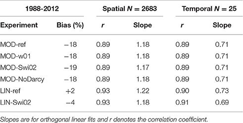
Table 3. Statistics of comparison between observed (Mote, 2014) and simulated annual melt day counts (see text for details) over the period 1988-2012.
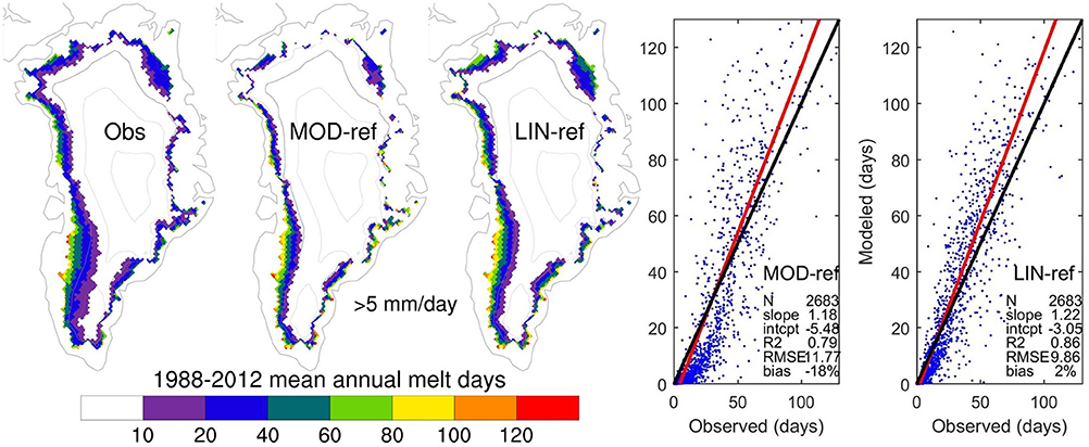
Figure 5. Comparison of 1988-2012 mean observed and modeled spatial distribution of annual melt day counts on the 25 km EASE-grid (see text for details). The maps show melt day counts in grid cells where both the observed and interpolated model fields have ice. The scatter plots include only points where either observations or model show melt. The black line is 1:1 and the red line is an orthogonal linear regression with statistics of the fit provided in the table. These are unitless except RMSE (m w.e.).
The MOD versions have ~18% too low long-term mean, ice sheet-wide melt day totals, while the LIN versions match observations closely (bias −4 to +2%). In all models, inter-annual variability in ice sheet-wide sums of melt day counts shows high correlation coefficient (~0.9) but with too shallow slope (~0.7) indicating that year-to-year differences are underestimated. The time-mean spatial pattern compares well in terms of correlation coefficient (~0.9) but with too steep slopes (~1.2), indicating too large differences between high and low melt day counts. Figure 5 illustrates the spatial patterns and statistics of the long-term average fields. The simulated patterns are similar to observations, with the main differences related to the steep spatial regression slopes: The model tends to have too few points with few melt days and too many points with many melt days.
Comparing the LIN and MOD models, correlation coefficients (spatial and temporal) and slopes (spatial and temporal) are very similar, while the LIN models have a better match in terms of mean, ice sheet-wide totals. Within the LIN and MOD groups the statistics do not give a clear winner.
Subsurface Temperature and Density
Figure 6 shows the 8–10 m depth observed and simulated subsurface temperature records at the percolation area site KAN-U 1840 m above sea level (Figure 2). The subsurface model is generally too warm at these depths during winter (Figure 6) due to some combination of (i) a surface temperature warm bias (not shown) and (ii) excessive retention in the top 5 m which heats the modeled subsurface during winter. Given that the Swi02 versions of the experiments (which have a fixed Swi of 0.02) display the same warm bias (not shown), excessive retained water is likely not the primary cause. In the early melt season, modeled temperatures are too low, indicating that the simulated wetting front advance is too slow. Once the wetting front has reached its maximum depth, the early-season cold bias subsides. The MOD-Swi02 and LIN-Swi02 experiments (not shown) allow, as discussed in the next section, a more rapid percolation to depth and the early melt season cold bias is less pronounced.
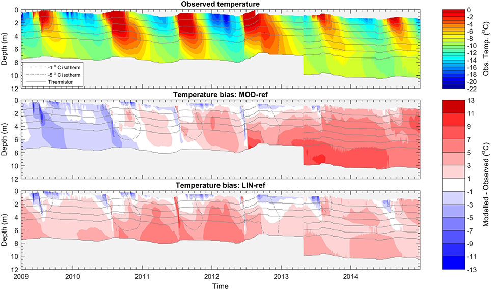
Figure 6. Comparison between modeled and observed subsurface temperatures at KAN-U for 2009-2014. The positions of the thermistors are indicated by solid gray lines. In the lower panels, showing the difference between modeled and observed temperatures, the −1 and −5°C isotherms from the top panel are repeated for reference. Major ticks mark the beginning of the year.
Two main differences between MOD-ref and LIN-ref at KAN-U are that the latter has a larger surface meltwater supply and produces a perched ice layer near 6 m depth beginning in summer 2011 (see Figure 8). Prior to that, the LIN experiment has a warm bias throughout the year below 5 m, while the MOD experiment is colder. In the summers following the ice layer formation in 2011, the LIN experiment is more in line with observations while the MOD experiment is too warm at depth. This difference agrees with the observed existence of an ice layer at the site in those years (Machguth et al., 2016a).
Figure 7 shows nine comparisons of simulated and observed density profiles from MOD-ref and LIN-ref. More cores are presented in Supplementary Figures S1 and S2, showing that the following discussions apply more generally. The model gives realistic density profiles in dry snow areas such as core 7551 in Figure 7. In these areas, MOD-ref and LIN-ref give similar results due to limited melt.
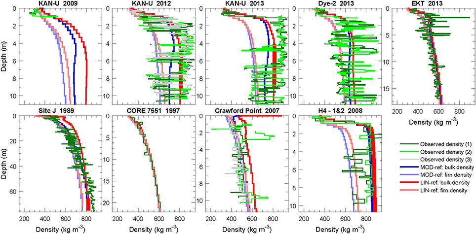
Figure 7. Comparison between observed (green, light green, and gray) and modeled (blue for MOD-ref, red for LIN-ref) density profiles. Modeled bulk densities, ρbulk (Equation 12), are shown in darker blue or red while dry firn density, ρs, is shown in lighter shades. Modeled densities exceeding pore close-off density (810 kg m−3) are shown with thicker lines.
In areas where more melt and refreezing occurs (all other panels in Figure 7), ice lenses of various thicknesses appear in the firn, and density profiles no longer increase monotonically with depth. At Site J for example, the smooth dry compaction profile is superimposed with sequences of higher and lower density peaks. Due to the model vertical resolution, it is not possible to recreate these thin features. However, agreement between the smoothed observed density (not shown) and modeled bulk density allows the model to accurately translate mass loss to surface lowering and calculate the thermal properties of the firn for that given resolution. On the other hand, the modeled firn density (shown in lighter shades) should match the ice-free sections of the observed density profile. In many cases, observed density profiles have low peak densities that are smaller than the modeled values, but with measurement uncertainty this overestimation of ice-free firn densities is perhaps less clear.
Wherever surface melt occurs, LIN-ref tends to give higher densities than MOD-ref because of the differences in meltwater input. In some cases it allows the LIN-ref model to reproduce observed ice lenses as shown with thick lines at KAN-U in 2012 and 2013. At other sites, such as Site J, LIN-ref clearly overestimates subsurface densities while MOD-ref fits the observed profile better.
The KAN-U core from 2009 only recorded densities to 1 m depth and stratigraphy down to 3 m and did not show any major ice lenses at shallow depth. In the cores from spring 2012, numerous ice layers are observed with some spatial variability (differences between multiple observed profiles). There, LIN-ref has reached pore close off at 5 m depth and replicates this densification process. The cores from spring 2013 show how the ice lens complexes had merged into a consistent ice layer. Accordingly the impermeable layer in LIN-ref also increased in thickness. A good spatial match is also visible on the EGIG line (first 15 panels in Supplementary Figure S2, ordered in decreasing altitude). The LIN-ref model reaches pore close off at the same sites where ice lenses and higher densities become frequent in the cores (from GGU163 to H2-1, differing only by 100 m in altitude). The MOD-ref model, however, reaches pore close off lower on this transect.
The observed density profiles at DYE-2 show a similar stratigraphy to what was observed at KAN-U before saturation of the near-surface firn and may potentially undergo a similar transformation. The EKT and Crawford Point cores also show increased ice features and density near the surface and can also potentially follow the same path. It is satisfactory to see the simulated density profile represent this near-surface densification due to increased refreezing in recent years. On the other end of the spectrum, sites like H4 show a stratigraphy where meltwater refreezing has filled most pore space except for isolated firn pockets at depth. Accordingly, simulated densities have reached pore close off at that site and surface melt is unable to percolate to depth.
Sensitivity Results
Subsurface Temperature and Water Profiles
Figure 8 shows the simulated development of the subsurface (uppermost 10 m) temperature at KAN-U in different experiments. The long term variability in MOD-ref indicates relatively cold conditions in the 1990s, a somewhat warmer subsurface in the 2000s and widespread near-temperate conditions throughout the top 10 m in the 2010s. The 2000s heating is even more pronounced in the MOD-Swi02 experiment which differs from MOD-ref only in the parameterization for Swi allowing considerably less water to be retained by capillary forces. As a result, surface meltwater is transferred more readily to depth thereby eroding the cold content. The MOD-NoDarcy experiment has the same irreducible saturation as MOD-ref but allows instantaneous downward percolation of water in excess of irreducible saturation. While this leads to differences between the two experiments on daily timescales (evident for liquid water content in the zoomed Figure 9), their resulting temperature structures are practically indistinguishable in Figure 8, even though daily values are, in fact, plotted.
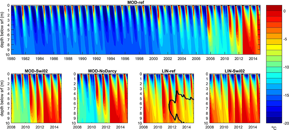
Figure 8. Daily mean temperature at KAN-U of the upper 10 m for 1980-2014 for MOD-ref and for 2008-2014 for other selected experiments. The black solid line marks the ρbulk = 810 kg m−3 contour indicating the presence of impermeable layers.
Using the LIN albedo results in a larger meltwater supply at the KAN-U site leading to higher subsurface temperatures than in the corresponding MOD experiments, i.e., LIN-ref is warmer than MOD-ref and LIN-Swi02 is warmer than MOD-Swi02. The deeper penetration of latent heating with Swi02 than with SwiCL is seen also for LIN in the summers 2008-2010. In July 2011, however, a drastic difference emerges in that the 810 kg m−3 contour becomes visible in LIN-ref indicating the presence of impermeable layers. The larger capacity of the SwiCL formulation to retain water allows enough of the percolating meltwater to refreeze and initiate an ice layer. As the season progresses with latent heat supply cut off from above, the ice layer can grow from below from retained meltwater supplied before it was formed. In the following winter, the layer is gradually cooled and buried by snow accumulation. However, when the 2012 meltwater front reaches the layer, the thickness grows again from above. The subsequent summers 2013 and 2014 add further mass to the layer from above (in accordance with observations; Machguth et al., 2016a) but not enough to compensate the winter burial. The net effect is therefore a downward motion of the ice layer after the end of the 2012 melt season.
Figure 9 illustrates the differences in subsurface liquid water content (L = pw/ps) arising due to the presence of the perched ice layer in LIN-ref but also to different choices of wh/wice and Darcy vs. NoDarcy. The presence of the ice layer in LIN-ref leads to an accumulation of liquid water on top which increases as long as supply from percolation continues. Two large melt events took place in July 2012 (Fausto et al., 2016b) during which this accumulation of liquid water is evident. In the intervening period, July 12 (day 194) to July 26 (day 208), runoff from the column lowers the liquid water level. The high levels of water in excess of the irreducible saturation leads to runoff from the time water starts accumulating atop the ice layer until late in the autumn season rather than being distributed over large depths as in the three left panels.
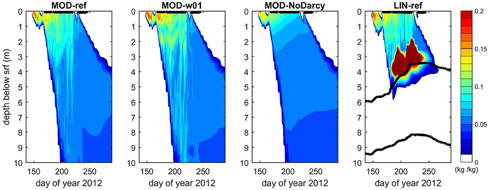
Figure 9. Mass liquid water content (L = pw/ps) of the upper 10 m at KAN-U for days 136–289 (May 15–Oct 15) of 2012 for selected experiments. The black solid lines mark the ρbulk = 810 kg m−3 contour indicating the presence of impermeable layers. In the rightmost panel, the accumulating water leads to values of up to 0.5, beyond the range of the color bar.
The distribution of liquid water content in MOD-ref vs. MOD-w01 shows the impact of reducing the hydraulic conductivity of the layers. Reduced conductivity in MOD-w01 slows the downward flow and allows for greater vertical gradients in liquid water to build up before being released. Such buildup of vertical gradients leads to a more intermittent downward flow pattern but not to formation of an impermeable layer. Opposite is the MOD-NoDarcy experiment in which excess water percolates instantaneously, leading to a gradual rather than intermittent evolution of the water field.
Since surface accumulation and percolation leads to simulated vertical shifting of mass, an ice layer effectively diffuses with time if no new mass is top-accreted after formation. A greater amount of meltwater is thus needed for the buildup of an ice layer that can survive the winter and still block percolation the next melt season. This could explain why MOD models do not form a sustainable ice layer at KAN-U.
Large-Scale Patterns of Perched Ice, Liquid Water, and Runoff
Figure 10 shows the distribution of perched ice layers over the years 2012-2014 along with the April 2014 distribution of perennial firn aquifers. Perched ice layers are identified from the three-dimensional field of ρbulk averaged over April: searching from the surface and downward, if one or more layers have ρbulk ≥810 kg m−3 followed by ρbulk <810 kg m−3, then that grid cell has an identified perched ice layer. Perched ice layers determined in this manner are present in a narrow band (typically 3–6 grid cells) going from the southwest up the west coast and around the north and northeast, and in some cases interrupted in the west and northwest by perennial firn aquifers.
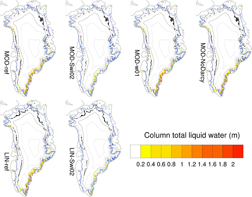
Figure 10. Distribution of ice layers (i.e., existence of layers with ρbulk ≥ 810 kg m−3 above less dense layers) in April of years 2012-2014 in black, and distribution of total column liquid water in April 2014 in reds. All panels include elevation contours (1000–3000 m a.s.l. in steps of 500 m with 2000 m a.s.l. highlighted) and outline of the contiguous ice sheet (blue).
The spatial distribution of perennial firn aquifers in the south matches qualitatively that found by Forster et al. (2014) in firn cores, airborne radar surveys and the regional climate model RACMO2. As in RACMO2, the modeled perennial firn aquifers consist entirely of water held within the irreducible saturation, since excess water has percolated further and refrozen or run off during autumn. The column total water content is thus tightly controlled by the parameterization of Swi and our Swi02 experiments are directly comparable to the RACMO2 results. As discussed by Kuipers Munneke et al. (2014), the existence of perennial firn aquifers requires high annual accumulation rates and moderate to high summer melt or rainfall. In addition to the areas in the southeast discussed by Forster et al. (2014), our model simulates these conditions also in several places in the west and northwest.
Comparing cases with SwiCL and Swi02 (i.e., MOD-ref vs. MOD-Swi02 and LIN-ref vs. LIN-Swi02), the perched ice layers are more widespread with SwiCL. The KAN-U site is, as illustrated in Figure 8, one such location where SwiCL, but not Swi02, allows an ice layer to emerge (in the LIN case). The higher retention of water in still cool near-surface layers apparently favors the formation of the perched ice layer.
Even though Figure 9 showed how daily variations in the subsurface water field and downward flow depend crucially on the implementation of hydraulic conductivity (MOD-ref vs. MOD-w01 vs. MOD-NoDarcy), it is apparently not important for the large-scale distribution of perched ice layers and perennial firn aquifers. It appears that the seasonal supply of meltwater, accumulation and irreducible saturation are important and not the exact timing of the downward flow on time-scales of days. This is a useful result for climate models, as it implies that capturing short-term variability is not as important as accurately capturing longer-term precipitation and snowpack processes.
Figure 11 shows differences in total runoff averaged over the years 2012-2014 arising due to the different model implementations. The top row shows the runoff in the MOD-ref and LIN-ref experiments and below is shown the difference between them. The LIN albedo promotes higher melting across the north, likely contributing to the more widespread occurrence of perched ice layers in that area in LIN-ref (Figure 10). In most of the west, south and east, however, the MOD experiment produces larger runoff rates. One exception is the green band inland of the yellow band in the west, indicating a higher runoff line in the LIN case.
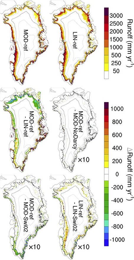
Figure 11. (Upper row) Annual runoff (averaged over years 2012-2014) for experiments MOD-ref and LIN-ref. (Lower rows) Runoff differences between selected experiments. The last three have been multiplied by 10 to aid visualization. All panels include elevation contours (1000–3000 m a.s.l. in steps of 500 m with 2000 m a.s.l. highlighted) and outline of the contiguous ice sheet.
The choice of albedo implementation is by far the most important factor for runoff. This is illustrated by the three remaining panels which have been multiplied by a factor of 10 for differences to appear. Again, the choice of Darcy vs. NoDarcy is particularly unimportant. In both the MOD (bottom left) and LIN (bottom right) cases, the choice of SwiCL vs. Swi02 has some impact. With exceptions, there is a general pattern of areas with perennial firn aquifers (south and southeast) giving less runoff with SwiCL and areas with perched ice layers (west and north) giving more runoff with SwiCL. This is to be expected since, in the absence of an ice layer, a higher Swi allows more water to be retained in the column and refrozen during the following winter. In the presence of an ice layer, the meltwater accumulating on top (as seen in Figure 9) leads to runoff rather than deep percolation.
Greenland-wide time-series of calendar-year total runoff and SMB are shown in Figure 12. Clearly discernible are the differences between the MOD and LIN cases, while the differences between SwiCL and Swi02 are very small. This is due both to the smallness of the differences in the lower row of Figure 11 (multiplied by a factor of 10) but also the competing effects from the perennial firn aquifer and perched ice layer areas. The MODIS-driven experiments employ an average 2000-2006 daily albedo climatology in the period before 2000. This reduces the inter-annual variability and leads to larger differences from the LIN experiments in runoff (and, consequently, SMB) in the pre-2000 period. In the post-2000 period with direct MODIS-derived albedos, there is better agreement on the variability.
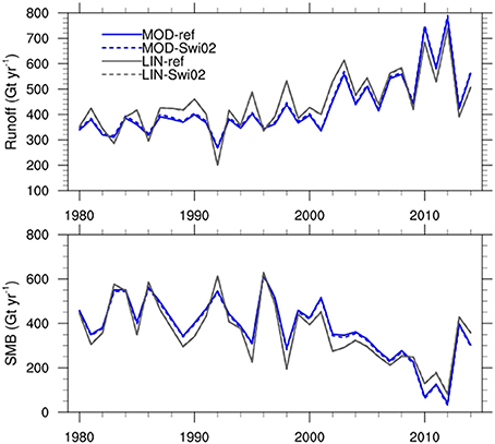
Figure 12. Greenland-wide annual runoff and SMB from selected experiments.
Conclusions
The subsurface scheme of the regional climate model HIRHAM5 has been extended to include firn densification, grain size growth, snow state-dependent hydraulic conductivity and irreducible water saturation as well as retention of water in excess of the irreducible saturation and superimposed ice formation. Sensitivity experiments have been performed to gauge both small- and large-scale effects of these additions as well as the impact of different parameterization choices.
The model results compare favorably with 68 ice core-derived annual net accumulation rates (spatial correlation coefficient of 0.90 and mean bias −5%). In the ablation area, simulated SMBs compare very well with 1041 observations with regression slopes of 0.97 and 0.95, and correlation coefficients of 0.86 and 0.75 for MOD-ref and LIN-ref, respectively. Mean biases are −3%, indicating only slightly underestimated net mass loss rates. The low mean bias is, however, partially due to a cancelation of under- and overestimates at high and low elevation sites. Splitting the sites between those above and below 700 m a.s.l. and weighting the resulting biases with the amount of runoff deriving from low vs. higher elevations results in weighted ice sheet-wide mass loss biases in the ablation area of −5 and −7% for MOD and LIN, respectively. These numbers do not depend significantly on other model choices (Darcy, Swi and wh/wice).
Comparing observed and simulated annual melt day counts shows that the spatial and temporal patterns of variability are reliably represented in the model, while it tends to underestimate the magnitude of inter-annual variability and overestimate that of spatial variability. As for the SMB comparison, the choice of albedo dominates the differences and the statistics do not allow for a best choice of the other model settings to be determined.
The mechanism for vertical flow (Darcy vs. NoDarcy and wh/wice set to 1 vs. 0.1) has an impact on short time-scale features of the subsurface liquid water field, but appears unimportant for the seasonal-scale temperature structure and for the large-scale mass balance field.
Two model choices do influence the subsurface temperature at KAN-U on longer time-scales, namely albedo and Swi. Prior to the formation of the ice lens, a larger meltwater production in LIN leads to a perennial warm bias below 5 m. Setting Swi to 0.02, rather than parameterized according to Coleou and Lesaffre (1998), allows water to percolate more readily to depth in the early melt season and reduces the cold bias otherwise present in the model at that time of year with both LIN and MOD. On the other hand, using the Coleou and Lesaffre (1998) parameterization in combination with LIN albedo allows for formation of an ice layer in agreement with observations (Figure 7 and Machguth et al., 2016a). This, in turn, shields the deeper part from latent heating from refreezing and reduces the warm bias at depth.
The model combinations without a perched ice layer at KAN-U do not produce runoff there over the 2009-2014 period, while LIN-ref generates 132 mm in 2010 and 583 mm in 2012. This agrees with the 690 ± 150 mm runoff in 2012 derived from comparison of spring 2012 and 2013 firn core stratigraphies by Machguth et al. (2016a) at KAN-U. This increase in runoff line altitude with the LIN-ref combination (also seen in Figure 11) is a direct consequence of the perched ice layer formation, and modeling this accurately appears crucial in a warming climate where more meltwater would be available in the percolation area. While the appearance of the perched ice layer at KAN-U is in line with observations, this does not necessarily imply that the LIN-ref combination is better than the others. As seen in Figure 10, perched ice layers do form also with MOD and Swi02 in different combinations; just not exactly at KAN-U.
Perennial firn aquifers occur in the south and southeast in patterns corresponding to those found by Forster et al. (2014) and continue up the west coast interrupted by areas with perched ice layers. These areas with perennial firn aquifers are not much impacted by the choice of SwiCL vs. Swi02, but the total amount of water in the aquifers is. This is because the perennial firn aquifer water consists entirely of water held within the irreducible saturation. In areas of perennial firn aquifers, SwiCL generally leads to less runoff because more water is held back against runoff in the summer and fall and remains available for refreezing in winter.
The fact that water exits the model domain once it runs off from a column may influence our results. If water instead flowed to neighboring grid columns (at the surface or at the depth from which it runs off), it would become part of the water budget of that cell. This could potentially increase the magnitude or areal extent of both perched ice layers and perennial firn aquifers. Addition of a representation of lateral flow and routing of water along with vertical piping could potentially alter the current conclusions and should be the focus of further developments.
As perched ice layers form, water which would otherwise have percolated and refrozen at deeper levels end up contributing to runoff instead. This is visible in large-scale runoff maps, but in a Greenland-wide accumulated sense, this is more or less negligible in the model's current climate. In general, the same is true for details of the percolation mechanism and retention parameterizations: they matter for local-scale subsurface temperature, snow, ice and water fields; but for the Greenland-wide runoff and SMB, the major impact is from the choice of albedo implementation. Whether the large-scale effects of perennial firn aquifers and perched ice layers will change in a warmer climate is not yet clear.
Author Contributions
PL led the development of the subsurface model, performed the subsurface experiments and led writing of the manuscript. RF, BV, and RM contributed to development of the subsurface model and RM performed the HIRHAM5 atmospheric model experiment. PL, BV, and JB performed comparisons of model output to observations. All authors contributed to discussions and writing of the manuscript.
Funding
This work is supported by the Retain project, funded by the Danish Council for Independent research (Grant no. 4002-00234).
Conflict of Interest Statement
The authors declare that the research was conducted in the absence of any commercial or financial relationships that could be construed as a potential conflict of interest.
The reviewer PA and handling Editor declared their shared affiliation, and the handling Editor states that the process nevertheless met the standards of a fair and objective review.
Acknowledgments
We are grateful to the three reviewers for their thorough and insightful input that lead to considerable improvements of the paper. We thank J. Harper, T. Kameda, M. Macferrin, H. Machguth, E. Mosley-Thompson, and D. van As for providing density profiles. The PARCA cores are available at http://research.bpcrc.osu.edu/Icecore/data/ and their collection was supported by NASA grants NAG5-5032 and 6817 to the Ohio State University, NASA grants NAG5-5031 and 6779 to the University of Arizona, and NASA grant NAGW-4248 and NSF/OPP grant 9423530 to the University of Colorado. The ACT campaigns were supported by NASA (grant NNX10AR76G), by the Greenland Analog Project (GAP), by the REFREEZE project, by the RETAIN project (DFF grant 4002-00234) and by the Programme for Monitoring of the Greenland Ice Sheet (PROMICE). PROMICE data are freely accessible at http://promice.org as is HIRHAM5 output at http://prudence.dmi.dk/data/temp/RUM/HIRHAM/GL2.
Supplementary Material
The Supplementary Material for this article can be found online at: https://www.frontiersin.org/article/10.3389/feart.2016.00110/full#supplementary-material
References
Ahlstrøm, A., Gravesen, P., Andersen, S., Van As, D., Citterio, M., Fausto, R., et al. (2008). A new programme for monitoring the mass loss of the Greenland ice sheet. Geol. Surv. Den. Greenland Bull. 15, 61–64. Available online at: http://www.geus.dk/DK/publications/geol-survey-dk-gl-bull/15/Documents/nr15_p61-64.pdf
Benson, C. S. (1962). Stratigraphic Studies in the Snow and Firn of the Greenland Ice Sheet. SIPRE, (CRREL) Research Report 70, reprinted with revisions by CRREL, 1996.
Box, J. E., Cressie, N., Bromwich, D. H., Jung, J.-H., van den Broeke, M., van Angelen, J. H., et al. (2013). Greenland ice sheet mass balance reconstruction. Part I: net snow accumulation (1600–2009). J. Climate 26, 3919–3934. doi: 10.1175/JCLI-D-12-00373.1
Box, J. E., Fettweis, X., Stroeve, J. C., Tedesco, M., Hall, D. K., and Steffen, K. (2012). Greenland ice sheet albedo feedback: thermodynamics and atmospheric drivers. Cryosphere 6, 821–839. doi: 10.5194/tc-6-821-2012
Braithwaite, R. J., W. Tad Pfeffer, Blatter, A., and Humphrey, N. F. (1992). “Meltwater refreezing in the accumulation area of the Greenland Ice Sheet, Pakitsoq Region, Summer 1991,” in Current Research, Greenland Geological Survey Report of Activities, Report No. 155, 13–17.
Braithwaite, R., Laternser, M., and Pfeffer, W. (1994). Variations of near-surface firn density in the lower accumulation area of the Greenland ice sheet, Pakitsoq, West Greenland. J. Glaciol. 40, 477–485.
Brun, E. (1989). Investigation on wet-snow metamorphism in respect of liquid-water content. Ann. Glaciol. 13, 22–26.
Calonne, N., Geindreau, C., Flin, F., Morin, S., Lesaffre, B., Rolland du Roscoat, S., et al. (2012). 3-D image-based numerical computations of snow permeability: links to specific surface area, density, and microstructural anisotropy. Cryosphere 6, 939–951. doi: 10.5194/tc-6-939-2012
Charalampidis, C., van As, D., Box, J. E., van den Broeke, M. R., Colgan, W. T., Doyle, S. H., et al. (2015). Changing surface–atmosphere energy exchange and refreezing capacity of the lower accumulation area, West Greenland. Cryosphere 9, 2163–2181. doi: 10.5194/tc-9-2163-2015
Christensen, O., Drews, M., Christensen, J., Dethloff, K., Ketelsen, K., Hebestadt, I., et al (2006). The HIRHAM Regional Climate Model, Version 5. Available online at: http://www.dmi.dk/fileadmin/Rapporter/TR/tr06-17.pdf
Church, J. A., Clark, P. U., Cazenave, A., Gregory, J. M., Jevrejeva, S., Levermann, A., et al. (2013). “Sea level change,” in Climate Change 2013: The Physical Science Basis. Contribution of Working Group I to the Fifth Assessment Report of the Intergovernmental Panel on Climate Change, eds T. F. Stocker, D. Qin, G.-K. Plattner, M. M. B. Tignor, S. K. Allen, J. Boschung, A. Nauels, Y. Xia, V. Bex, and P. M. Midgley (Cambridge; New York, NY: Cambridge University Press), 1137–1216. Available online at: www.climatechange2013.org
Cogley, J. G., Hock, R., Rasmussen, L. A., Arendt, A. A., Bauder, A., Braithwaite, R. J., et al. (2011). Glossary of Glacier Mass Balance and Related Terms. IHP-VII Technical Documents in Hydrology No. 86, IACS Contribution No. 2, UNESCO-IHP, Paris.
Colbeck, S. (1974). The capillary effects on water percolation in homogeneous snow. J. Glaciol. 13, 85–97.
Colbeck, S. (1975). A theory for water flow through a layered snowpack. Water Resour. Res. 11, 261–266. doi: 10.1029/WR011i002p00261
Coleou, C., and Lesaffre, B. (1998). Irreducible water saturation in snow: experimental results in a cold laboratory. Ann. Glaciol. 26, 64–68.
Cuffey, K. M., and Paterson, W. S. B. (2010). The Physics of Glaciers. Amsterdam: Elsevier Science, 704.
Dee, D. P., Uppala, S. M., Simmons, A. J., Berrisford, P., Poli, P., Kobayashi, S., et al. (2011). The ERA-Interim reanalysis: configuration and performance of the data assimilation system. Q. J. R. Meteorol. Soc. 137, 553–597. doi: 10.1002/qj.828
de la Peña, S., Howat, I. M., Nienow, P. W., van den Broeke, M. R., Mosley-Thompson, E., Price, S. F., et al. (2015). Changes in the firn structure of the western Greenland Ice Sheet caused by recent warming. Cryosphere 9, 1203–1211. doi: 10.5194/tc-9-1203-2015
Dumont, M., Brun, E., Picard, G., Michou, M., Libois, Q., Petit, J.-R., et al. (2014). Contribution of light-absorbing impurities in snow to Greenland's darkening since 2009. Nat. Geosci 7, 509–512. doi: 10.1038/ngeo2180
Eerola, K. (2006). About the performance of HIRLAM version 7.0. HIRLAM Newslett. 51, 93–102. Available online at: http://hirlam.org/index.php/hirlam-documentation/doc_view/473-hirlam-newsletter-no-51-article14-eerola-performance-hirlam7-0
Fausto, R. S., van As, D., Box, J. E., Colgan, W., and Langen, P. L. (2016a). Quantifying the surface energy fluxes in south Greenland during the 2012 high melt episodes using in situ observations. Front. Earth Sci. 4:82. doi: 10.3389/feart.2016.00082
Fausto, R. S., van As, D., Box, J. E., Colgan, W., Langen, P. L., and Mottram, R. H. (2016b). The implication of nonradiative energy fluxes dominating Greenland ice sheet exceptional ablation area surface melt in 2012. Geophys. Res. Lett. 43, 2649–2658. doi: 10.1002/2016GL067720
Fettweis, X. (2007). Reconstruction of the 1979–2006 Greenland ice sheet surface mass balance using the regional climate model MAR. Cryosphere 1, 21–40. doi: 10.5194/tc-1-21-2007
Forster, R. R., Box, J. E., van den Broeke, M. R., Miege, C., Burgess, E. W., van Angelen, J. H., et al. (2014). Extensive liquid meltwater storage in firn within the Greenland ice sheet. Nat. Geosci. 7, 95–98. doi: 10.1038/ngeo2043
Gascon, G., Sharp, M., Burgess, D., Bezeau, P., and Bush, A. B. G. (2013). Changes in accumulation-area firn stratigraphy and meltwater flow during a period of climate warming: Devon Ice Cap, Nunavut, Canada. J. Geophys. Res. Earth Surf. 118, 2380–2391. doi: 10.1002/2013jf002838
Gregory, J. M., White, N. J., Church, J. A., Bierkens, M. F. P., Box, J. E., van den Broeke, M. R., et al. (2013). Twentieth-century global-mean sea level rise: is the whole greater than the sum of the parts? J. Climate 26, 4476–4499. doi: 10.1175/JCLI-D-12-00319.1
Gregory, S. A., Albert, M. R., and Baker, I. (2014). Impact of physical properties and accumulation rate on pore close-off in layered firn. Cryosphere 8, 91–105. doi: 10.5194/tc-8-91-2014
Harper, J., Humphrey, N., Pfeffer, W. T., Brown, J., and Fettweis, X. (2012). Greenland ice-sheet contribution to sea-level rise buffered by meltwater storage in firn. Nature 491, 240–243. doi: 10.1038/nature11566
Hirashima, H., Yamaguchi, S., Sato, A., and Lehning, M. (2010). Numerical modeling of liquid water movement through layered snow based on new measurements of the water retention curve. Cold Regions Sci. Technol. 64, 94–103. doi: 10.1016/j.coldregions.2010.09.003
Howat, I. M., de la Peña, S., van Angelen, J. H., Lenaerts, J. T. M., and van den Broeke, M. R. (2013). Brief Communication “Expansion of meltwater lakes on the Greenland Ice Sheet.” Cryosphere 7, 201–204. doi: 10.5194/tc-7-201-2013
Humphrey, N. F., Harper, J. T., and Pfeffer, W. T. (2012). Thermal tracking of meltwater retention in Greenland's accumulation area. J. Geophys. Res. Earth Surf. 117:F01010. doi: 10.1029/2011jf002083
Janssens, I., and Huybrechts, P. (2000). The treatment of meltwater retention in mass-balance parameterisations of the Greenland ice sheet. Ann. Glaciol. 31, 133–140. doi: 10.3189/172756400781819941
Kameda, T., Narita, H., Shoji, H., Nishio, F., Fujii, Y., and Watanabe, O. (1995). Melt features in ice cores from Site J, southern Greenland: some implications for summer climate since AD 1550. Ann. Glaciol. 21, 51–58.
Katsushima, T., Kumakura, T., and Takeuchi, Y. (2009). A multiple snow layer model including a parameterization of vertical water channel process in snowpack. Cold Regions Sci. Technol. 59, 143–151. doi: 10.1016/j.coldregions.2009.09.002
Keegan, K. M., Albert, M. R., McConnell, J. R., and Baker, I. (2014). Climate change and forest fires synergistically drive widespread melt events of the Greenland Ice Sheet. Proc. Natl. Acad. Sci. U.S.A. 111, 7964–7967. doi: 10.1073/pnas.1405397111
Koenig, L. S., Miège, C., Forster, R. R., and Brucker, L. (2014). Initial in situ measurements of perennial meltwater storage in the Greenland firn aquifer. Geophys. Res. Lett. 41, 81–85. doi: 10.1002/2013GL058083
Kuipers Munneke, P. M., Ligtenberg, S. R., van den Broeke, M. R., van Angelen, J. H., and Forster, R. R. (2014). Explaining the presence of perennial liquid water bodies in the firn of the Greenland Ice Sheet. Geophys. Res. Lett. 41, 476–483. doi: 10.1002/2013GL058389
Langen, P. L., Mottram, R. H., Christensen, J. H., Boberg, F., Rodehacke, C. B., Stendel, M., et al. (2015). Quantifying energy and mass fluxes controlling Godthåbsfjord freshwater input in a 5 km simulation (1991–2012). J. Climate. 28, 3694–3713. doi: 10.1175/jcli-d-14-00271.1
Lefebre, F., Gallée, H., van Ypersele, J.-P., and Greuell, W. (2003). Modeling of snow and ice melt at ETH Camp (West Greenland): a study of surface albedo. J. Geophys. Res. 108:4231. doi: 10.1029/2001jd001160
Ligtenberg, S. R. M., Helsen, M. M., and van den Broeke, M. R. (2011). An improved semi-empirical model for the densification of Antarctic firn. Cryosphere 5, 809–819. doi: 10.5194/tc-5-809-2011
Lucas-Picher, P., Wulff-Nielsen, M., Christensen, J. H., Ağalgeirsdóttir, G., Mottram, R., and Simonsen, S. B. (2012). Very high resolution regional climate model simulations over Greenland: identifying added value. J. Geophys. Res. 117:D02108. doi: 10.1029/2011jd016267
Machguth, H., MacFerrin, M., van As, D., Box, J. E., Charalampidis, C., Colgan, W., et al. (2016a). Greenland meltwater storage in firn limited by near-surface ice formation. Nature Clim. Change 6, 390–393. doi: 10.1038/nclimate2899
Machguth, H., Thomsen, H. H., Weidick, A., Ahlstrøm, A. P., Abermann, J., Andersen, M. L., et al. (2016b). Greenland surface mass-balance observations from the ice-sheet ablation area and local glaciers. J. Glaciol. 62, 861–887. doi: 10.1017/jog.2016.75
Mosley-Thompson, E., McConnell, J. R., Bales, R. C., Li, Z., Lin, P.-N., Steffen, K., et al. (2001). Local to regional-scale variability of annual net accumulation on the Greenland ice sheet from PARCA cores. J. Geophys. Res. 106, 33839–33851. doi: 10.1029/2001JD900067
Mote, T. L. (2007). Greenland surface melt trends 1973–2007: evidence of a large increase in 2007. Geophys. Res. Lett. 34, L22507. doi: 10.1029/2007GL031976
Mote, T. L. (2014). MEaSUREs Greenland Surface Melt Daily 25km EASE-Grid 2.0. Boulder, CO: NASA DAAC at the National Snow and Ice Data Center. doi: 10.5067/MEASURES/CRYOSPHERE/nsidc-0533.001
Mote, T. L., and Anderson, M. R. (1995). Variations in snowpack melt on the Greenland ice sheet based on passive microwave measurements. J. Glaciol. 41, 51–60.
Oerlemans, J., and Knap, W. (1998). 1 year record of global radiation and albedo in the ablation zone of Morteratschgletscher, Switzerland. J. Glaciol. 44, 231–238.
Parry, V., Nienow, P., Mair, D., Scott, J., Hubbard, B., Steffen, K., et al. (2007). Investigations of meltwater refreezing and density variations in the snowpack and firn within the percolation zone of the Greenland ice sheet. Ann. Glaciol. 46, 61–68. doi: 10.3189/172756407782871332
Pfeffer, W. T., Meier, M. F., and Illangasekare, T. H. (1991). Retention of Greenland runoff by refreezing: implications for projected future sea level change. J. Geophys. Res. 96, 22117–22124. doi: 10.1029/91JC02502
Polashenski, C., Courville, Z., Benson, C., Wagner, A., Chen, J., Wong, G., et al. (2014). Observations of pronounced Greenland ice sheet firn warming and implications for runoff production. Geophys. Res. Lett. 41:2014GL059806. doi: 10.1002/2014GL059806
Reeh, N. (1989). Parameterization of melt rate and surface temperature on the Greenland ice sheet. Polarforschung 59, 113–128.
Reijmer, C. H., van den Broeke, M. R., Fettweis, X., Ettema, J., and Stap, L. B. (2012). Refreezing on the Greenland ice sheet: a comparison of parameterizations. Cryosphere 6, 743–762. doi: 10.5194/tc-6-743-2012
Roeckner, E., Bäuml, G., Bonaventura, L., Brokopf, R., Esch, M., Giorgetta, M., et al. (2003). The Atmospheric General Circulation Model ECHAM5. Part I: Model Description. Available online at: http://www.mpimet.mpg.de/fileadmin/publikationen/Reports/max_scirep_349.pdf
Shimizu, H. (1970). Air permeability of deposited snow. Contribut. Instit. Low Temp. Sci. A22, 1–32.
Tedesco, M., Doherty, S., Fettweis, X., Alexander, P., Jeyaratnam, J., and Stroeve, J. (2016). The darkening of the Greenland ice sheet: trends, drivers, and projections (1981–2100). Cryosphere 10, 477–496. doi: 10.5194/tc-10-477-2016
van Angelen, J. H., Lenaerts, J. T. M., Lhermitte, S., Fettweis, X., Kuipers Munneke, P., van den Broeke, M. R., et al. (2012). Sensitivity of Greenland Ice Sheet surface mass balance to surface albedo parameterization: a study with a regional climate model. Cryosphere 6, 1175–1186. doi: 10.5194/tc-6-1175-2012
van Angelen, J. H. M., Lenaerts, J. T., van den Broeke, M. R., Fettweis, X., and van Meijgaard, E. (2013). Rapid loss of firn pore space accelerates 21st century Greenland mass loss. Geophys. Res. Lett. 40, 2109–2113. doi: 10.1002/grl.50490
van Angelen, J. H., van den Broeke, M. R., Wouters, B., and Lenaerts, J. T. M. (2014). Contemporary (1960–2012) evolution of the climate and surface mass balance of the Greenland Ice Sheet. Surv. Geophysi. 35, 1155–1174. doi: 10.1007/s10712-013-9261-z
van As, D., Box, J., and Fausto, R. (2016). Challenges of quantifying meltwater retention in snow and firn: an expert elicitation. Front. Earth Sci. 4:101. doi: 10.3389/feart.2016.00101
van As, D., Fausto, R., Colgan, W., Box, J., and PROMICE Project Team (2013). Darkening of the Greenland ice sheet due to the meltalbedo feedback observed at PROMICE weather stations. Geol. Sur. Den. Greenland Bull. 28, 69–72. Available online at: http://www.geus.dk/publications/bull/nr28/nr28_p69-72.pdf
van den Broeke, M., Bamber, J., Ettema, J., Rignot, E., Schrama, E., van de Berg, W. J., et al. (2009). Partitioning recent greenland mass loss. Science 326, 984–986. doi: 10.1126/science.1178176
van Genuchten, M. T. (1980). A closed-form equation for predicting the hydraulic conductivity of unsaturated soil. Soil Sci. Soc. Am. J. 44, 892–898. doi: 10.2136/sssaj1980.03615995004400050002x
Vernon, C. L., Bamber, J. L., Box, J. E., van den Broeke, M. R., Fettweis, X., Hanna, E., et al. (2013). Surface mass balance model intercomparison for the Greenland ice sheet. Cryosphere 7, 599–614. doi: 10.5194/tc-7-599-2013
Vionnet, V., Brun, E., Morin, S., Boone, A., Faroux, S., Le Moigne, P., et al. (2012). The detailed snowpack scheme Crocus and its implementation in SURFEX v7.2. Geosci. Model Dev. 5, 773–791. doi: 10.5194/gmd-5-773-2012
Wever, N., Schmid, L., Heilig, A., Eisen, O., Fierz, C., and Lehning, M. (2015). Verification of the multi-layer SNOWPACK model with different water transport schemes. Cryosphere 9, 2271–2293. doi: 10.5194/tc-9-2271-2015
Wright, A. P., Wadham, J. L., Siegert, M. J., Luckman, A., Kohler, J., and Nuttall, A. M. (2007). Modeling the refreezing of meltwater as superimposed ice on a high Arctic glacier: a comparison of approaches. J. Geophys. Res. 112:F04016. doi: 10.1029/2007JF000818
Yamaguchi, S., Katsushima, T., Sato, A., and Kumakura, T. (2010). Water retention curve of snow with different grain sizes. Cold Regions Sci. Technol. 64, 87–93. doi: 10.1016/j.coldregions.2010.05.008
Yen, Y. (1981). Review of Thermal Properties of Snow, Ice and Sea Ice. Hanover, NH: United States Army Cold Regions Research and Engineering Laboratory. Report number: CRREL Report 81-10.
Keywords: liquid water percolation in firn, regional climate model, HIRHAM5 subsurface scheme, Greenland ice sheet runoff, Greenland ice sheet surface mass balance, Greenland ice sheet perched ice layers, Greenland ice sheet perennial firn aquifer
Citation: Langen PL, Fausto RS, Vandecrux B, Mottram RH and Box JE (2017) Liquid Water Flow and Retention on the Greenland Ice Sheet in the Regional Climate Model HIRHAM5: Local and Large-Scale Impacts. Front. Earth Sci. 4:110. doi: 10.3389/feart.2016.00110
Received: 04 October 2016; Accepted: 22 December 2016;
Published: 12 January 2017.
Edited by:
Marco Tedesco, NASA Goddard Institute for Space Studies-Columbia University, USAReviewed by:
Michiel Van Den Broeke, Utrecht University, NetherlandsXavier Fettweis, University of Liège, Belgium
Patrick Alexander, NASA Goddard Institute for Space Studies, USA
Copyright © 2017 Langen, Fausto, Vandecrux, Mottram and Box. This is an open-access article distributed under the terms of the Creative Commons Attribution License (CC BY). The use, distribution or reproduction in other forums is permitted, provided the original author(s) or licensor are credited and that the original publication in this journal is cited, in accordance with accepted academic practice. No use, distribution or reproduction is permitted which does not comply with these terms.
*Correspondence: Peter L. Langen, pla@dmi.dk